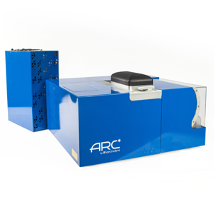
Spectradyne's nCS1TM and ARCTM
Microfluidic resistive pulse sensing (MRPS)
Microfluidic resistive pulse sensing (MRPS) is the microfluidic cousin of resistive pulse sensing or RPS. The main difference is that the analysis chamber in RPS is replaced by a disposable microfluidic cartridge, where different cartridge models are designed to have different size apertures, allowing a wider range of particle sizes to be analyzed. This means that the cartridge chosen for the particle size analysis can be optimized for the particle sizes expected in the sample.
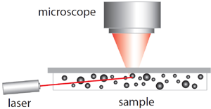
Spectradyne's nCS1TM and ARCTM employ microfluidic resistive pulse sensing using disposable microfluidic cartridges. By using state-of-the art microfluidic fabrication technology, we have shrunk the critical particle sensing constriction used in traditional RPS by a factor of 100 or so, from a few tens of microns in diameter to a few hundred nanometers. This allows us to detect much smaller particles using MRPS than is possible using RPS. A schematic of a microfluidic cartridge is shown below. The microfluidic cartridges include a 3 μL reservoir for the analyte, on-board filters, ports for voltage-biasing the analyte, a sense electrode, a fluid resistor and the critical MRPS aperture or nanoconstriction, through which particles flow one at a time. The analyte, which could be blood serum, diluted or full-strength phosphate-buffered saline, or any conducting fluid, is electrically biased by the voltage-bias electrodes, causing an electrical current to flow through the analyte, the fluidic resistor and the aperture. When a particle suspended in analyte flows through the aperture, it changes the electrical resistance of the constriction by occluding part of the current, by an amount proportional to the ratio of the nanoparticle volume to that of the aperture, just as in RPS. Individual particles thus give changes in the sense voltage proportional to their volume, allowing them to be counted and sized. The much smaller apertures available in Spectradyne's microfluidic cartridges allow much smaller particles to be detected.
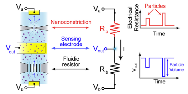
The disposable MRPS cartridge includes ports for voltage bias Va and Vb, a microfluidic nanoconstriction or aperture Ra and a fluidic resistor Rb, The voltage bias causes a current I to flow, setting the voltage Vout of the sense electrode. Particles flowing through the aperture change the aperture resistance in time (top right), thereby causing measurable changes in the sense voltage Vout. These changes are proportional to particle volume, so each particle's volume is measured individually.
You can read more about microfluidic resistive pulse sensing elsewhere on our website:
- An overview of our technology
- Compare with the other particle size analyzer technologies
- Spectradyne's MRPS allows measurements over a wide range of concentrations
- Specifications for Spectradyne's nCS1TM
- An article published in American Laboratory is available here
- A technical article that appeared in Nature Nanotechnology is available here
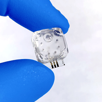
A microfluidic cartridge at the heart of Spectradyne's MRPS technology.
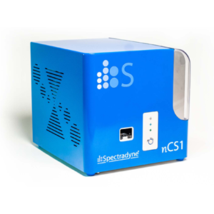
Spectradyne's nCS1TM, which performs measurements using a microfluidic cartridges.